| impulse_and_momentum_lab-.doc |
Purpose
the purpose of this lab is to measure a cart’s momentum change and compare it to the impulse it
receives. Compare average and peak forces in impulses.
receives. Compare average and peak forces in impulses.
Materials
CBL
2 interface
dynamics cart and track
TI Graphing Calculator
clamp
Vernier
Force Sensor
elastic cord
Vernier Motion Detector
DataMate program
string
500-g mass
2 interface
dynamics cart and track
TI Graphing Calculator
clamp
Vernier
Force Sensor
elastic cord
Vernier Motion Detector
DataMate program
string
500-g mass
1. Measure the mass of your dynamics cart and record the value in the Data
Table.
2. Place the track on a level surface. Confirm that the track is level
by placing the low-friction
cart on the track and releasing it from rest. It
should not roll. If necessary, adjust the track.
3. Attach the elastic cord
to the cart and then the cord to the force sensor. Choose a cord length
so that the cart can roll freely with the cord slack for most of the track length, but be stopped
by the cord before it reaches the end of the track. Clamp the
Force Sensor so that the cord,
when taut, is horizontal and in line with the
cart’s motion.
4. Place the Motion Detector beyond the other end of the
track so that the detector has a clear
view of the cart’s motion along the
entire track length. When the cord is stretched to
maximum extension the
cart should not be closer than 0.4 m to the detector.
5. Connect the Student
Force Sensor to Channel 1 of the CBL 2 interface. Connect the Motion
Detector to the SONIC/DIG or SONIC/DIG 1 input of the interface. Use the
black link cable to
connect the interface to the TI Graphing Calculator.
Firmly press in the cable ends.
6. Turn on the calculator and start the
DATAMATE program. Press CLEAR to reset the program.
7. If CH 1 displays the
Force Sensor and its current reading, skip the remainder of this step. If
not, set up DATAMATE for the Force Sensor manually (the interface will
recognize the Motion
Detector automatically). To do this,
a. Select SETUP
from the main screen.
b. Press ENTER to select CH1
c. Choose FORCE from
the SELECT SENSOR list.
d. Choose STUDENT FORCE for your force sensor.
e.
Select OK to return to the main screen.
8. Zero the Force Sensor.
a.
Select SETUP from the main screen.
b. Select ZERO.
c. Select CH 1 from the
SELECT CHANNEL menu.
d. Remove all force from the Force Sensor.
e. When
the reading on the calculator screen is stable, press ENTER to record the zero
condition.
9. Set up the calculator and interface for data
collection.
a. Select SETUP from the main screen.
b. Press to select MODE
and press ENTER .
c. Select TIME GRAPH from the SELECT MODE screen.
d.
Select CHANGE TIME SETTINGS.
e. Enter “0.02” as the time between samples in
seconds. (Use “0.05” for the TI-73 and 83.)
f. Enter “150” as the number of
samples. (Use “50” for the TI-73 and 83.)
g. Select OK twice to return to the
main screen.10. Practice releasing the cart so it rolls toward the Motion
Detector, bounces gently, and returns
to your hand. The Force Sensor must
not shift and the cart must stay on the track. Arrange the
cord and string
so that when they are slack they do not interfere with the cart motion. You
may need to guide the string by hand, but be sure that you do not apply any
force to the cart
or Force Sensor. Keep your hands away from between the
cart and the Motion Detector.
11. Select START to take data. As soon as you
hear the interface beep, roll the cart as you
practiced in the previous
step.
12. Study your graphs to determine if the run was useful:
a. Press
ENTER to see the force graph.
b. Inspect the force data. If the peak is
flattened, then the applied force is too large. Repeat
your data collection
with a lower initial speed.
c. Press ENTER to return to the graph selection
screen.
d. Press to select DIG-DISTANCE.
e. Press ENTER to see the
distance graph.
f. Confirm that the Motion Detector detected the cart
throughout its travel. If there is a noisy
or flat spot near the time of
closest approach, then the Motion Detector was too close to
the cart. Move
the Motion Detector away from the cart, and repeat your data collection.
g.
Press ENTER to return to the graph selection screen, and select MAIN
SCREEN.
h. To collect further data, return to Step 11.
13. Once you have
made a run with good distance and force graphs, analyze your data. To test the
impulse-momentum theorem, you need the velocity before and after the
impulse. To find
these values,
a. Select ANALYZE from the main
screen.
b. Select STATISTICS from the ANALYZE OPTIONS.
c. Select
DIG-VELOCITY from the SELECT GRAPH screen.
d. Now you can select a portion of
the velocity graph for averaging. Using the and
cursor keys, move the lower
bound cursor to the left side of the approximately constantand negative-velocity
region. Press ENTER .
e. Now set the upper bound: Move the cursor to the
right edge of the approximately
constant- and negative-velocity region.
Press ENTER .
f. Read the average velocity before the collision (vi) from
the calculator. Record the value in
your Data Table.
g. Press ENTER to
return to the ANALYZE OPTIONS screen.
h. In the same manner, determine the
average velocity just after the bounce (vf) and record
this positive value
in your Data Table.
14. (Calculus version) Now record the value of the
impulse.
a. Select INTEGRAL from the ANALYZE OPTIONS.
b. Select
CH1-FORCE(N) from the select graph screen.
c. Now you can select a portion of
the force graph for integration. Using the cursor keys,
move the cursor to
just before the impulse begins, where the force becomes non-zero.
Press
ENTER .
d. Now move the cursor to the right edge of the impulse, where the
force returns to zero.
Press ENTER .
e. Calculus tells us that the
expression for the impulse is equivalent to the integral of the
force vs.
time graph, or
Data
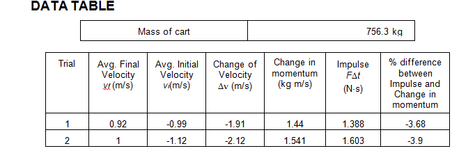
First trial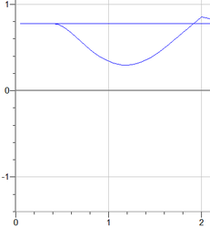
distance vs time
|
|
Second Trial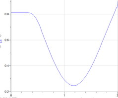
distance vs time
|
|
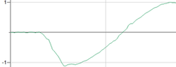
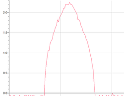
Data Analysis
At the beginning of the lab in trial one we had a percent difference of 3.68% and in trial 2 we had a
percent difference of 3.9%. This percent error was due to an an error in our force sensor. we could not calibrate the force sensor to be zero. The force sensor continued to calibrate at a small negative number.
The small negative value that we were given as what should have been our zero value it caused our force vs time value to be slightly lower on the graph.
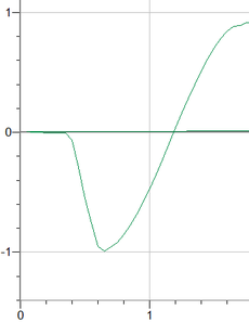
We solved the max forces of the trials to be 2.01 for trial one and 2.26 for trial two. The average forces for the trials were 1.388 for trial one and 1.78 for trial two.
In trial one there was a time interval of 1.0 seconds and trial two had an interval of 0.9 seconds.
percent difference of 3.9%. This percent error was due to an an error in our force sensor. we could not calibrate the force sensor to be zero. The force sensor continued to calibrate at a small negative number.
The small negative value that we were given as what should have been our zero value it caused our force vs time value to be slightly lower on the graph.
We solved the max forces of the trials to be 2.01 for trial one and 2.26 for trial two. The average forces for the trials were 1.388 for trial one and 1.78 for trial two.
In trial one there was a time interval of 1.0 seconds and trial two had an interval of 0.9 seconds.
Conclusion
The main idea of this lab was to compre the change in momentum of the cart with the change in impulse of the cart. The change in momentum should be equal to the impulse of an action. Although in our lab, our results were a little less than 5% off. This error could have partially been due to air resistance and friction, but was mostly because of the force sensor failing to calibrate at zero. Finally, the last part of the lab was to compare the average forces to the maximum forces in each of the trials.
